Fractal curve app, taxonomy, book, and gallery

Greetings fractal curve fans. I’ve been busy, on many levels – as we like to say in the fractal curves business. I made a fractal curve generator app that uses only complex integer math. Check it out:

This was made to test my hypothesis: that plane-filling fractal curves could not only be categorized using complex integers; they could also be generated with complex integers. Basing this method on complex integers helps to explore number theory without a messy mantissa. The conclusion is that a plane-filling fractal curve can be generated using only addition, multiplication, and conjugation of complex integers. This is explained in my new book, the Family Tree of Fractal Curves.

 

 

 

 

 

 

 

 

Here’s a collection of plane-filling curves illustrating this taxonomy:

I also updated the fractal curve art gallery. Enjoy!

A plane-filling curve that sweeps the pinwheel tiling

Adam Goucher, who writes a blog called Complex Projective 4-Space, got me motivated several years ago to work on a taxonomy of plane-filling curves, based on complex integers. I’ve just completed a new book on the subject, called The Family Tree of Fractal Curves. A free version is also available on the Internet Archive. Adam looked at an earlier version of the draft, and made an interesting observation, relating my scheme for generating plane-filling curves to the pinwheel tiling – which is a non-periodic tiling.

image above from this web site: http://www.quadibloc.com/math/til04.htm

Imagine having an unlimited number of tiles that are right triangles, with sides of length 1, 2, and √5. The tiles can be assembled in unlimited ways – as long as adjacent edges are the same length. 

The pinwheel tiling can be represented in my plane-filling curve taxonomy as part of the G(25,0) family (see page 73 of the book) by way of a reflection, a rotation, and a scaling by √5. The third and fourth segments of the generator are overlapping.

In the picture below, the top row shows three iterations (progressive subdivision) of the triangle. Below that is the genetic code for the plane-filling curve, whose generator is shown in the box as a collection of Gaussian integers (line segments in the square lattice). All of the segments have norm 5 (Euclidean distance = √5). At the bottom of the picture is the result of iterating the generator.

 

It’s always exciting to see geometry ideas come together like this. So much interesting math, research, and design is happening right now with tilings and plane-filling curves (which are of course related!)

A ramified curve

Since the generator for this curve is self-overlapping (two of the five segments overlap), it is more “dense” than the self-avoiding variety of curves. Mandelbrot referred to these curves as “ramified”. One way to visualize self-overlapping and self-contacting curves is to render them with splines (rounding off the corners). This helps to reveal the sweep of the curve:

Aperiodic tilings (and curves) are stimulating to the eye and brain, perhaps because of the peculiar mix of symmetry and asymmetry.

Plane-filling curves, when related to tilings like these, provide a scheme for ordering the tiles. It opens up a new way to think about what may otherwise seem like a disordered mess.

Adam suggested that this tiling could be rendered using a node-replacement curve (in addition to an edge-replacement curve). Node replacement curves have a more obvious relation to plane-filling tilings in that they can be described as a way of connecting the centers of adjacent tiles. The ordering of connections is the same as that of edge-replacement.

I am sure that there is a lot more to say on this subject. If you are a fellow fractal geek, you might have something to add. Please chime in!

-Jeffrey

A Complete Taxonomy of Plane-filling Curves

I am in the process of completing several years of work in developing a complete taxonomy of plane-filling curves. There are infinitely many plane-filling curves, but most of the ones you are familiar with can be found among the first nine families:

Some of these were introduced in Mandelbrot’s famous book. They are constructed using “edge-replacement” (Mandelbrot called it “Koch construction”).

“Edge-replacement curves” are to be contrasted with “node-replacement curves” such as the Hilbert Curve. (I explain the difference between these two techniques in this article).

Have you ever wondered if there is a relationship between the classic Dragon Curve and Mandelbrot’s Amazing self-avoiding Snowflake Sweep?

Have you ever wondered why some space-filling curves are self-avoiding, while others touch themselves all over? Below is the Gosper Curve and Dragon of Eve (a self-avoiding curve I discovered in the 1980’s):

Both the Dragon of Eve and another curve I discovered (below) each have generators with only three segments. These constitute the simplest generators (in terms of segment count) that afford self-avoiding curves:

Notice that these curves occupy two kinds of lattice: square and triangular (sometimes called “hexagonal lattice”). I mentioned this to Adam Goucher, and asked him if he had any insights abut the special properties of these curves, in terms of how they relate to the lattices that they occupy. He said that these properties can be understood in terms of the Gaussian integers (square lattice) and Eisenstein integers (triangular lattice).

Thank you Adam! What amazing discoveries poured in after thinking of these curves in this way. I have begun to think of a plane-filling curve as an ordered sum of integers (each segment is an integer “added” to the previous segment in the list). The endpoint is an integer in the plane which represents the family for that curve.

Here are just a few of the hundreds of amazing curves I have fished out of the deep sea, in the process of developing this taxonomy. (Some of the self-touching curves have been smoothed-out with splines to reveal the beautiful sweep of its path as it fills the body).

 

I will be adding more on this subject over the year. Meanwhile, come visit fractalcurves.com.

Fractal Curves in Gaussian and Eisenstien Integer Lattices

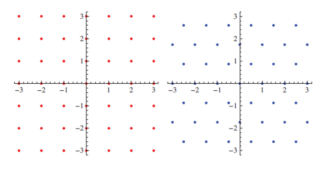
I have been working on a taxonomy of space-filling curves in the square and triangular lattices. I came across Adam Goucher’s blog: Complex Projective 4-Space. I asked Adam what he thought of my proposed fractal curve families and he told me that I should study the Gaussian and Eisenstein integers. The image below shows Gaussian integers (red dots) and Eisenstein integers (blue dots).

So cool! Adam pointed me to a whole new world of discovery that I am still unraveling and unfolding to this day.

I will not get into the details of Gaussian and Eisenstein integers here, except to say that they are sets of complex numbers occupying square and triangular lattices respectively. (You can click on the links provided and follow the search to any level of detail you wish).

They can be seen as two-dimensional versions of the one-dimensional number line of integers that we are all so familiar with.

Like their familiar one-dimensional counterpart, the Gaussian and Eisenstein integers form an integral domain: the rules of addition and multiplication apply, and these operations always result in a new number which is within the domain. Gaussian and Eisenstein integers have their own unique prime number and composite number personalities – which make for a fascinating study – including how they relate to families of plane-filling curves.

The Koch Curve and it’s Squarish cousin occupy triangular and square grids, respectively. And each has a “spine” that traverses exactly three units.

In these two lattices, all distances of grid points from the origin (0+0i) are square roots of integers (Euclidian norm).

Squaring the Euclidian norm gives us the field norm , the integer that we use to denote the fractal family. It is either prime or composite.

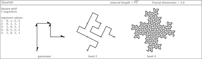
Here are some examples of plane-filling curves that occupy the square lattice:

Example 1 (also discovered by Carbajo)

Example 2 (Mandelbrot’s “Quartet”)

Example 3: (a Root 13 self-avoiding curve)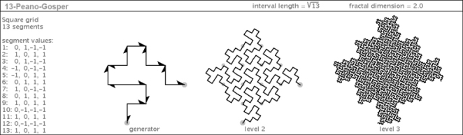

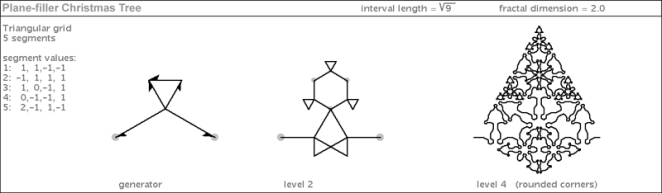
And here are some examples of plane-filling curves that occur in the triangular lattice:

Example 4: (a curve I discovered)

Example 5: (a member of the Root 7 family)

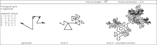
Example 6: (a member of the triangle Root 9 family)

Check out the generators of these curves (shown at the left of each diagram). You may have noticed that some of them consist of line segments of differing lengths. These represent members of composite fractal families: their spines traverse a distance that is equal to the square root of a composite number in the domain. (Examples 1, 4, and 6 are composite).

The members of “prime” families (examples 2, 3, and 5 above) can only have segments of length 1. Consequently, as they are iterated to create higher-level teragons, with more fractal detail, the texture becomes more even and smooth. The composite curves – on the other hand – have varying density within their flesh, which increases in variety as they are iterated.

This is awesome: it’s another way to show the recursive complexity of composite numbers. And if you ask me (and Greg Chaitin), the composite numbers are way more interesting than the primes!

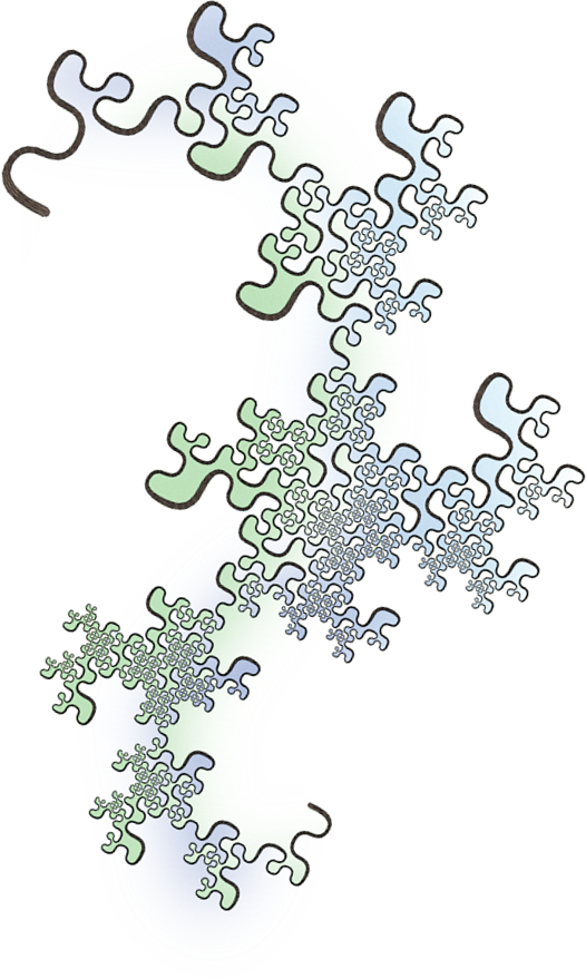
Here’s a plane-filling curve of the root-8 family. Since 8 = 2^3, this family contains interesting variants of the famous dragon curve, which is a member of the root 2 family. This example has the corners rounded for aesthetics. It shows some of the variation in scale within its flesh.

I’ll be posting more as discoveries are made. Stay tuned!

-Jeffrey