“Outside-In” – On Doug McKenna’s Generalized Hilbert curves

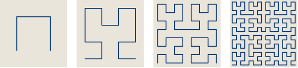
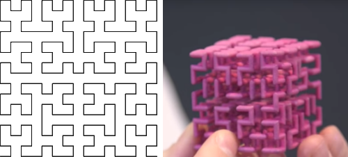
Here’s one of the fractal curves described by Doug McKenna in his new interactive electronic book, Hilbert Curves -Outside-In and Inside-Gone, available on iPad/iPhone.

How would you describe the outline of this shape? That’s a loaded question.

————-

The depth of Doug McKenna’s fractal curviness is not only demonstrated in his latest works; he was developing fundamental designs and curve concepts at the dawn of the Fractal Age.

Of course, Peano, Koch, Sierpinski, and others had already published their now-famous curves long ago. But the craft of making fractal curves truly got its start in the late 60’s, when the Dragon curve was discovered, and then through the 70’s – around the time when Benoit Mandelbrot was working on his thesis on fractals. Some of the people who were hired to design fractal illustrations under Mandelbot’s direction (including Doug) got overshadowed. This is partially due to Mandelbrot’s well-deserved clout, but it is also because of Mandelbrot’s notorious habit of not giving proper attribution to key people on his team.

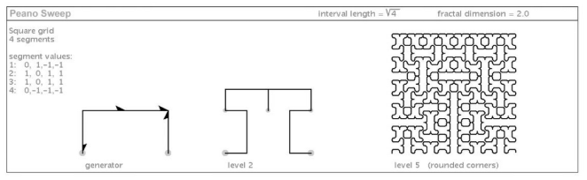
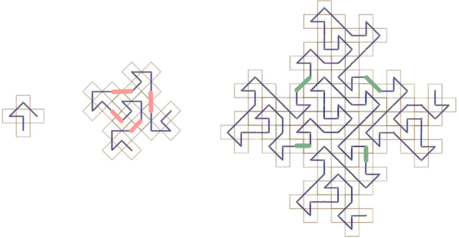
I want to shine some light on one of the earliest inventors of the field. Here’s another picture; this one is from one of Doug’s papers.

As you can see, the motif at left is multiplied many times to fill the interior of the shape to the right of it. It consists of a single self-avoiding curve. The third iteration, shown to the right of that, is also self-avoiding (although the image resolution is too coarse to show this).

There is a certain kind of fuzziness that accumulates on the horizontal edges at each level of iteration, as if ever-smaller forms of moss were growing on the backs of larger forms of moss. Okay; choose your own metaphor, but you get the idea. This is a way of thinking about fractal boundaries – as layers of fuzz.

And fuzz…comes in many forms!

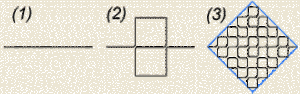
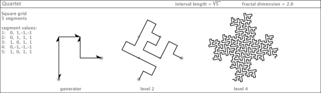
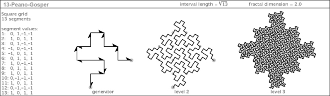
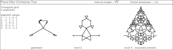
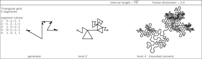
I came across this mind-bending concept while trying to describe the boundaries of some curves I had discovered. My latest book illustrates three plane-filling curves that have different degrees (and kinds) of ruggedness in their boundaries:

The boundary of the first curve is straight (not counting the corners). The more times it is iterated, the more that straightness gets expressed. The fractal dimension of its boundary is 1. In contrast, the second curve has a rather convoluted boundary (with a much higher fractal dimension).  Not only does the boundary pinch itself off in accumulating wasp-waist points at every iteration, but parts of its boundary appear to get closer with every iteration, perhaps self-contacting at infinity. This curve is not filling a simple-boundary topological unit in the plane; it is splitting itself into an infinity of body parts and even leaving holes (tremas) as it iterates.

But the topological weirdness gets more weird when you try to describe the boundary of the third curve. This curve, when sufficiently iterated, turns itself into a sort of “plane-filling gasket” (fyi – Gasket fractals are well-studied and illustrated). Forget about trying to identify its interior from its exterior – it’s impossible with this curve.

Well, seeing Doug’s new curves reminded me of this paradoxical nature of fractal curve boundaries.

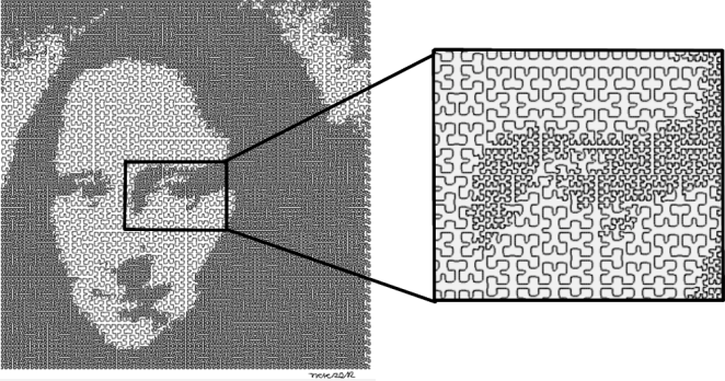
As soon as you start to think of the boundary of a fractal curve as a fractal in itself, things start to get really meta. This is one of the concepts highlighted in Doug’s new book, which, extends the Hilbert curve into an infinite hierarchy of ever-complexifying variations.

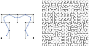
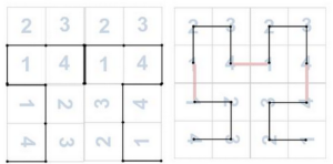
In the 1994 conference proceedings, The Lighter Side of Mathematics, there is paper written by Doug, called SquaRecurves, E-Tours, Eddies, and Frenzies: Basic Families of Peano Curves on the Square Grid. This paper introduces some of his earlier explorations. Here is an illustration from that paper:

Doug identified several classes of related curves that are all self-avoiding. I reconstructed some of his curves for my book. Here are a few of those illustrations.

These boundaries are fairly easy to see. In fact the E-curve, fills a square, like the Hilbert curve. But with so much potential variation, it doesn’t take much genetic manipulation to turn a square-filling curve into a wild and crazy beast.

Wikipedia occasionally lies. Here’s one such lie: “a space-filling curve is a curve whose range contains the entire 2-dimensional unit square.”

Such a lack of imagination…as well as being wrong.

I challenge anyone to tell me that the following space-filling curve is a square.

If that’s a square, then I’m a Klein bottle.

This curve is an example of Doug’s new “half-domino curves“. It can tesselate with a 180-rotated version of itself to create something at least more square-like, for those of you who are uncomfortable with exterior fuzz.

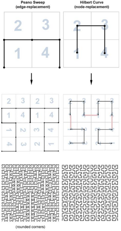
McKenna’s newer curves extend the basic concept of the Hilbert curve, making it just one instance of a larger class of curves.

Even within the square, there is an infinite variety of plane-filling sweeps. But some of these curves bust out of their square homes and push the fractal dimension of their boundaries to the point of them becoming their own space-filling curves. That’s meta!

On filling the Koch Snowflake

The hardback cover of my edition of The Fractal Geometry of Nature has a shiny gold pattern embossed on it:

The curve that separates the two color regions in this image is called the “Snowflake Sweep”. It is one of my favorite plane-filling curves. This was Mandelbrot’s solution for filling the interior of the Koch Snowflake.

Here is a schematic I made that describes the generator of this curve, using my taxonomy:

I have always been impressed with the cleverness of this curve; in particular, the way that the 5th segment (which is longer than the others) determines the central copy of the generator. There is always one copy of the generator in the middle of the curve, and it is always the largest, no matter how many levels the curve has been iterated.

I had made several attempts at coming up with a different way of filling the Koch snowflake. But all I could come up with were curves that incompletely fill the Koch Snowflake – that is: with curves having a fractal dimension less than 2.

My attempts were a failure in terms of plane-filling the Koch snowflake with a fractal curve of dimension 2. But in terms of aesthetics, I was not disappointed. To celebrate my “failure” I rendered these curves with icy, snowy colors:

While my attempts to fill the Koch snowflake with a fractal curve were unsuccessful, I was actually successful at filling it with a branching fractal:

(I plan to describe this branching solution in a future blog post).

In the process of doing research for my book, I came across a paper by Dekking and Dekking, which describes an attempt at filling the Koch snowflake. Here are some of the illustrations from that paper:

Dekking’s goal was to fill the curve evenly; that is, with all segments having the same length and thus avoiding the effect of uneven filling that appears in Mandelbrot’s original curve. Although the uneven filling accounts for its aesthetics, it is an interesting mathematical problem to fill a finite graph so that every edge is covered. This is known as an Eulerian Path.

Well, Dekking was indeed able to come up with an evenly-plane-filling curve, but the area that the curve fills has many tremas (holes): it does not fill the whole interior of the Koch Snowflake.

So, this leads to a question: is there any way to fill the Koch Snowflake with a continuous curve, other than with Mandelbrot ‘s original solution?

It would appear that the answer is…

Yes…

…but it requires a generalization of the edge-replacement method, using the power of L-systems.

I recently had the pleasure and honor of meeting (and drawing fractals with…) some of the most clever and creative people working in this area, at the Bridges conference in Linz. Among them were Douglas McKenna (who developed some of the earliest curves which appear in Mandelbrot’s book), and Jörg Arndt, who has been developing a new family of plane-filling curves, along with his colleague Julia Handl.

Jörg came up with a clever way of filling the Koch Snowflake using an L-system to determine a curve that conforms to an Archimedean tiling:

“WTF?” I said to Jörg: there are SQUARES in that tiling! How can a square possibly be a part of this solution? According to my world-view, the Snowflake Sweep conforms to the triangular grid. This tiling with three kinds of polygons – one being a square – was just counterintuitive to me.

However, I started to shift my world-view a bit, and it began to make sense. Imagine extracting a chunk of this tiling with the approximate shape of the Koch Snowflake. There are a few ways to do this:

You could specify a larger chunk and it would correspond to a higher iteration of the Snowflake – the larger the chunk, the more closely the boundary approximates the Snowflake.

So, where does the curve fit in? Jörg used two generators in his L-system – each generator corresponds to a continuous path of several segments in the grid – all segments having the same length. Jörg may publish his L-system rules soon, with a full explanation. In the meanwhile, here are some images collected from this web page:

I am still not clear on how this particular tiling allows the Snowflake to be generated; I am so accustomed to thinking of this curve as corresponding to the regular triangle grid. As an experiment, I tried overlaying a low-iteration version of Jörg’s curve on teragon 2 of the original sweep, and then again on a different scaling and translation of a triangular grid. Here is what I came up with:

There are some interesting symmetries here. Food for thought. Can you see any relationships that are revealing?

I suspect that with every iteration of this curve, the central (larger) segment corresponds to a new triangular grid having a different translation, rotation, and/or scaling.

Perhaps these curiosities are related to the way the Koch Snowflake tessellates with itself, as illustrated in the colorful design below by Robert Fathauer: (note how the large red snowflake and the smaller orange snowflakes combine to make a larger snowflake – with the same shape.

Jörg has found many other cool curves that conform to non-regular tilings like this, and they are described in this paper:

Plane-filling curves on all uniform grids

https://arxiv.org/abs/1607.02433.

It is fun (in a nerdy, fractally way) to be watching this exploration unfold.

Fractal curve app, taxonomy, book, and gallery

Greetings fractal curve fans. I’ve been busy, on many levels – as we like to say in the fractal curves business. I made a fractal curve generator app that uses only complex integer math. Check it out:

This was made to test my hypothesis: that plane-filling fractal curves could not only be categorized using complex integers; they could also be generated with complex integers. Basing this method on complex integers helps to explore number theory without a messy mantissa. The conclusion is that a plane-filling fractal curve can be generated using only addition, multiplication, and conjugation of complex integers. This is explained in my new book, the Family Tree of Fractal Curves.

 

 

 

 

 

 

 

 

Here’s a collection of plane-filling curves illustrating this taxonomy:

I also updated the fractal curve art gallery. Enjoy!

African Fractal Trees in Linz, Austria

Stefan Pautze and I were ordering meals at an African restaurant in Linz Austria, during the Bridges conference. He and I had each presented our art/math research. (Stefan has produced some beautiful fractal animations). We were drawing fractal curves on napkins (…as one does…at Bridges). Stefan looked up and said, “Hey look. Fractal trees!” The waitress was kind enough to allow us to photograph her apron.

The Gosper Dragon

One of the most famous and amazing plane-filling curves of all time is the Gosper curve.

In the process of developing a taxonomy of plane-filling curves, I discovered several relatives of the Gosper curve in a large family of curves that correspond to the Eisenstein integer 3+1ω. This is described in my new book, The Family Tree of Fractal Curves. A few of the curves of that family are shown here:

These curves have some things in common. For one thing, they all have “Gosper skin” – their boundaries have the same rugged fractal profile if you zoom in to the boundary at arbitrarily high magnification, and they have the same fractal dimension.

Below is a progression of teragons, starting with the initiator.

The illustration below shows how the Gosper Dragon corresponds to the same initiator as the Gosper curve. The initiator is a vector originating from the origin of the complex plane and ending at the Eisenstein integer 3+1ω, which has a norm of 7.

Notice that the Gosper Dragon is a self-avoiding curve, just like the Gosper curve. But it appears to cover a larger area. My conjecture is that this is because it has lower curvature: the sum of the absolute values of the angles in the generator is 420 in the Gosper curve; while it is only 360 in the Gosper Dragon. In other words, the Gosper curve has tighter turns (on average) in its sweeping path than the Gosper Dragon.

Notice in the illustration below that the “belly” of the Gosper Dragon (shown in purple) is a smaller version of the Gosper curve. The the head and tail (shown in green) are incomplete chunks of the Gosper curve.

Many kinds of self-similarity are common in the family. Three Gosper Dragons can be tessellated to compose a single Gosper curve:

Could there be more dragon-like relatives in this family to be discovered? Some new finding just may show up at fractalcurves.com. in the next few months. Stop by for a visit some time soon!

A plane-filling curve that sweeps the pinwheel tiling

Adam Goucher, who writes a blog called Complex Projective 4-Space, got me motivated several years ago to work on a taxonomy of plane-filling curves, based on complex integers. I’ve just completed a new book on the subject, called The Family Tree of Fractal Curves. A free version is also available on the Internet Archive. Adam looked at an earlier version of the draft, and made an interesting observation, relating my scheme for generating plane-filling curves to the pinwheel tiling – which is a non-periodic tiling.

image above from this web site: http://www.quadibloc.com/math/til04.htm

Imagine having an unlimited number of tiles that are right triangles, with sides of length 1, 2, and √5. The tiles can be assembled in unlimited ways – as long as adjacent edges are the same length. 

The pinwheel tiling can be represented in my plane-filling curve taxonomy as part of the G(25,0) family (see page 73 of the book) by way of a reflection, a rotation, and a scaling by √5. The third and fourth segments of the generator are overlapping.

In the picture below, the top row shows three iterations (progressive subdivision) of the triangle. Below that is the genetic code for the plane-filling curve, whose generator is shown in the box as a collection of Gaussian integers (line segments in the square lattice). All of the segments have norm 5 (Euclidean distance = √5). At the bottom of the picture is the result of iterating the generator.

 

It’s always exciting to see geometry ideas come together like this. So much interesting math, research, and design is happening right now with tilings and plane-filling curves (which are of course related!)

A ramified curve

Since the generator for this curve is self-overlapping (two of the five segments overlap), it is more “dense” than the self-avoiding variety of curves. Mandelbrot referred to these curves as “ramified”. One way to visualize self-overlapping and self-contacting curves is to render them with splines (rounding off the corners). This helps to reveal the sweep of the curve:

Aperiodic tilings (and curves) are stimulating to the eye and brain, perhaps because of the peculiar mix of symmetry and asymmetry.

Plane-filling curves, when related to tilings like these, provide a scheme for ordering the tiles. It opens up a new way to think about what may otherwise seem like a disordered mess.

Adam suggested that this tiling could be rendered using a node-replacement curve (in addition to an edge-replacement curve). Node replacement curves have a more obvious relation to plane-filling tilings in that they can be described as a way of connecting the centers of adjacent tiles. The ordering of connections is the same as that of edge-replacement.

I am sure that there is a lot more to say on this subject. If you are a fellow fractal geek, you might have something to add. Please chime in!

-Jeffrey

A Complete Taxonomy of Plane-filling Curves

I am in the process of completing several years of work in developing a complete taxonomy of plane-filling curves. There are infinitely many plane-filling curves, but most of the ones you are familiar with can be found among the first nine families:

Some of these were introduced in Mandelbrot’s famous book. They are constructed using “edge-replacement” (Mandelbrot called it “Koch construction”).

“Edge-replacement curves” are to be contrasted with “node-replacement curves” such as the Hilbert Curve. (I explain the difference between these two techniques in this article).

Have you ever wondered if there is a relationship between the classic Dragon Curve and Mandelbrot’s Amazing self-avoiding Snowflake Sweep?

Have you ever wondered why some space-filling curves are self-avoiding, while others touch themselves all over? Below is the Gosper Curve and Dragon of Eve (a self-avoiding curve I discovered in the 1980’s):

Both the Dragon of Eve and another curve I discovered (below) each have generators with only three segments. These constitute the simplest generators (in terms of segment count) that afford self-avoiding curves:

Notice that these curves occupy two kinds of lattice: square and triangular (sometimes called “hexagonal lattice”). I mentioned this to Adam Goucher, and asked him if he had any insights abut the special properties of these curves, in terms of how they relate to the lattices that they occupy. He said that these properties can be understood in terms of the Gaussian integers (square lattice) and Eisenstein integers (triangular lattice).

Thank you Adam! What amazing discoveries poured in after thinking of these curves in this way. I have begun to think of a plane-filling curve as an ordered sum of integers (each segment is an integer “added” to the previous segment in the list). The endpoint is an integer in the plane which represents the family for that curve.

Here are just a few of the hundreds of amazing curves I have fished out of the deep sea, in the process of developing this taxonomy. (Some of the self-touching curves have been smoothed-out with splines to reveal the beautiful sweep of its path as it fills the body).

 

I will be adding more on this subject over the year. Meanwhile, come visit fractalcurves.com.

Is there a 3D Gosper curve?

The Gosper curve is one of the most amazing and satisfying plane-filling curves.

The Gosper curve is a self-avoiding, plane-filling fractal curve containing 7^n segments (where n is the order of the teragon). It approximates the shape of a hexagon. It is named after the mathematician William Gosper.

Like all plane-filling curves generated using a deterministic recursive algorithm, the Gosper curve can be mapped to a tiling. In this case, the tile is the hexagon. As you increase the order of the teragon, the number of line segments – and thus hexagons – increases. And the boundary becomes more rugged. Below at right is an image of the Gosper boundary, created by the tiling of seven “rep-tiles“, each self-similar to the whole shape.

Counting Pennies

The regular hexagon is similar to the circle in the sense that the close-packing of circles forms a hexagonal arrangement. Imagine having 343 (7^3) pennies arranged on a table. If you try to push them together into the smallest area you can,  you might end up approximating the shape of the Gosper curve.

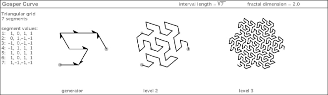
There are many ways to count a bunch of pennies. In this case you could count them in the order of the Gosper curve’s sweep. Since it is recursive, you could pause every 7 pennies to catch your breath. And you could also pause every 49 pennies for longer breaks. Between each break, you will have traced out a low-order Gosper curve.

On To the Third Dimension

Now, what if we extend this idea to three dimensions? Well, consider the close-packing of spheres. In the case of spheres, there are 12 spheres that can surround a single sphere, making a clump with a total of 13 spheres.

And…just as close-packing circles correspond to the tiling hexagon, 3D circles (spheres) correspond to the tiling rhombic dodecahedron.

Rhombic dodecahedra can be tiled infinitely, leaving no gaps and having no overlaps. This brings us to the big question: might there be a 3D spacefilling curve that can be drawn within a volume which is the union of 13^n rhombic dodecahedra? In other words…

Is there such a thing as a 3D Gosper Curve?
Now, to be fair…asking this question is a bit like asking, “Is there a 3D Mandelbrot Set?” The boring but true answer is no, of course not! …because the canonical Mandelbrot Set is by definition a 2D object. Also, the mathematical properties of complex numbers do not translate into 3D.

You may be able to find a 4D analog of the Mandelbrot Set by skipping the third dimension and jumping over to the fourth dimension. (Hamilton tried in vain to find a 3D analog of complex numbers. And this led him to the next dimension – where he discovered quaternions). FYI – the Mandebrot Set’s 2D nature didn’t stop explorers from trying to find a higher being. And in the process, what they found was something extraordinary: The Mandelbulb.

Now, back to the 3D Gosper curve. Is there is anything we can call a “3D Gosper curve”? To earn that title, it would have to have some fundamental attributes in common with the Gosper curve. This is what I had in mind as I set out to discover this elusive higher being. As a template, I chose the tessellation of 13 rhombic dodecahedra, because it it similar to the tessellation of 7 hexagons.

I posed my question to mathematician Henry Segerman. Just as you can tile seven hexagons (one in the middle surrounded by six), you can analogously tile thirteen rhombic dodecahedra (one in the middle surrounded by twelve). But can you then take 13 of these shapes and tile them into a larger blob of 13^3 dodecs? To explore the problem, Henry came up with the following images that he created using Rhino. After only two levels of recursion, he came to the conclusion that they probably do not tile   !!!!  

I asked Henry to send me the file for this 3D model, and then asked my colleague Barry Stump to fabricate it on his 3D printer. Here’s what Barry came up with:

Well, three of these shapes tessellate. But we need to tessellate 13 of them with the same symmetry as the original 13 unit tiles – to see with our own eyes and feel with our own hands – before we can be sure.

Before even asking whether a space-filling curve can be drawn that traverses each dodecahedron, I needed to determine whether the overall space can recursively tile without limit, and with no gaps or overlaps. If the answer is negative, then there is no use in asking about the curve, because it would not extend infinitely, as in the case of the canonical Gosper curve.

The jury is out. But it’s not looking good. A proof that it cannot be done would be better than nothing.

On Filling Fractal Dimensions 

It is well known that the Hilbert curve can be extended into 3D, as was shown in The Algorithmic Beauty of Plants. (Dave Fracchia did the raytrace rendering of this on an old SGI machine – back in the day 🙂 Anyway, there are still many unanswered questions. I have a feeling that certain people (like Henry) will have key insights about this. Henry has created physical versions of the Hilbert curve. This is an example of a 3D space-filling curve that has a direct analog in 2D. So what is it about the Hilbert curve that allows it to extend into 3D?

My original line of inquiry was this: think of the Hilbert curve in terms of tiling squares. The 2D Hilbert curve maps a line of length 2 to a square of area 2^2 = 4. The 3D Hilbert curve maps a line of length 2 to a cube of volume 2^3 = 8. The idea of the Hilbert curve as progressive squaring is described in my blog post comparing the Hilbert curve with the Peano Sweep:

Could the same logic be used with other shapes? Other than the cube, the logical 3D tessellating shape in my mind is the rhombic dodecahedron. But it appears not to tesselate recursively to create rep-tiles. My hope was (and still is) that there exists a tiling polyhedron within which one can fit a line between vertices having a length equal to the cube root of 13, and that 13 of these would tile to form a volume of 13. But am I misguided by looking for the cube root? Perhaps I need to consider the square root? (The Euclidean distance).

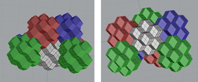
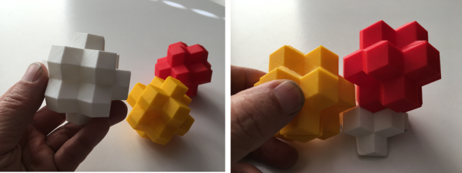
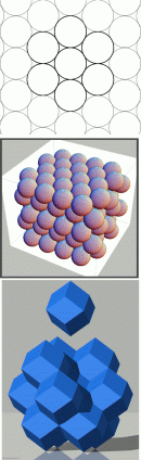
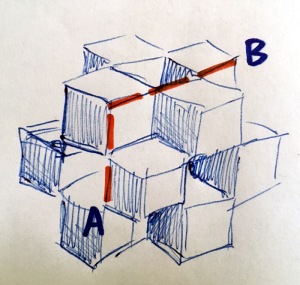
Here’s a picture I drew of 13 unit cubes representing rhombic dodecahedra. (BTW – if you stellate each face of a cube by adding a square pyramid, it becomes a rhombic dodecahedron. And if you start with a “3D checkerboard” of 13 cubes, like I have drawn, the result is 13 tessellating rhombic dodecahedra. Cool, eh? Now, look at red lines in the drawing. the distance from A to B happens to be the square root of 13 (assuming unit cubes).

A line drawn from A to B might be analogous to the line drawn within the hexagon in the image at the beginning of this article. Am I missing something?

I have a feeling that there are answers right around the corner. And it may be that I am simply asking the wrong questions!

And it still may be that we have to jump over the third dimension to the land of quaternions to get the right answers. There, we might find a new realm of hyper-space-filling curves – living among the integer quaternions – analogous to the Gaussian and Eisenstein integers, which are integral domains in which number theory can be used to make sense of space-filling curves.

The Hilbert Curve is Similar to the Peano Sweep

Imagine an upward surge of fluid like this:

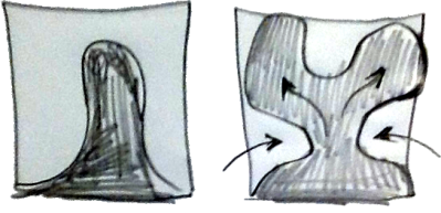
As the dark fluid surges upward, the light-colored fluid around it gets pulled inward, creating a “neck” as shown above at right, and the dark fluid bifurcates at the top. You can compare this shape to the generators for the Hilbert curve and the Peano Sweep. Since these are plane-filling fractal curves, they carry this dance of surging fluids down to smaller and smaller levels, until the fluid regimes are completely mixed. Below are the first few iterations of this mixing.

Hilbert Curve

Peano Sweep

The Hilbert curve is conveniently self-avoiding: no matter how much the fluids mix, the curve never touches itself. But the Peano Sweep has overlapping segments. This can be alleviated using a technique to separate the overlaps, which makes it topologically similar to the Hilbert curve, in terms of its intricate branching structure.

This comparison is described in more detail here, and it is illustrated below.

One key difference is that the Hilbert curve is a “node replacement curve” while the Peano Sweep is an “edge-replacement curve”. Edge-replacement curves were used by Mandelbrot in the introduction to fractals in his book. (He referred to this as Koch construction).

The Hilbert curve and Peano Sweep both conform to a four-square tiling scheme in which the main square is replaced with four smaller squares, and the two bottom ones are rotated inward.

Notice that the Hilbert curve requires connective links at every iteration. This is a required step for node-replacement curves, as shown in this variation of Mandelbrot’s Quartet that I discovered:

There are many more examples of plane-filling curves that use different tiling schemes, including a series of curves that Peano discovered, using nine inner-squares.

Several people have used plane-filling curves like this to define an image as a squiggly line. Imagine drawing the Mona Lisa with only one line, and the line gets more squiggly when it needs to cover a darker area:

(the above image is based on the Peano Sweep and it is explained here)

Stay tuned for more adventures with plane-filling curves!

-Jeffrey

 

Fractal Curves in Gaussian and Eisenstien Integer Lattices

I have been working on a taxonomy of space-filling curves in the square and triangular lattices. I came across Adam Goucher’s blog: Complex Projective 4-Space. I asked Adam what he thought of my proposed fractal curve families and he told me that I should study the Gaussian and Eisenstein integers. The image below shows Gaussian integers (red dots) and Eisenstein integers (blue dots).

So cool! Adam pointed me to a whole new world of discovery that I am still unraveling and unfolding to this day.

I will not get into the details of Gaussian and Eisenstein integers here, except to say that they are sets of complex numbers occupying square and triangular lattices respectively. (You can click on the links provided and follow the search to any level of detail you wish).

They can be seen as two-dimensional versions of the one-dimensional number line of integers that we are all so familiar with.

Like their familiar one-dimensional counterpart, the Gaussian and Eisenstein integers form an integral domain: the rules of addition and multiplication apply, and these operations always result in a new number which is within the domain. Gaussian and Eisenstein integers have their own unique prime number and composite number personalities – which make for a fascinating study – including how they relate to families of plane-filling curves.

The Koch Curve and it’s Squarish cousin occupy triangular and square grids, respectively. And each has a “spine” that traverses exactly three units.

In these two lattices, all distances of grid points from the origin (0+0i) are square roots of integers (Euclidian norm).

Squaring the Euclidian norm gives us the field norm , the integer that we use to denote the fractal family. It is either prime or composite.

Here are some examples of plane-filling curves that occupy the square lattice:

Example 1 (also discovered by Carbajo)

Example 2 (Mandelbrot’s “Quartet”)

Example 3: (a Root 13 self-avoiding curve)

And here are some examples of plane-filling curves that occur in the triangular lattice:

Example 4: (a curve I discovered)

Example 5: (a member of the Root 7 family)

Example 6: (a member of the triangle Root 9 family)

Check out the generators of these curves (shown at the left of each diagram). You may have noticed that some of them consist of line segments of differing lengths. These represent members of composite fractal families: their spines traverse a distance that is equal to the square root of a composite number in the domain. (Examples 1, 4, and 6 are composite).

The members of “prime” families (examples 2, 3, and 5 above) can only have segments of length 1. Consequently, as they are iterated to create higher-level teragons, with more fractal detail, the texture becomes more even and smooth. The composite curves – on the other hand – have varying density within their flesh, which increases in variety as they are iterated.

This is awesome: it’s another way to show the recursive complexity of composite numbers. And if you ask me (and Greg Chaitin), the composite numbers are way more interesting than the primes!

Here’s a plane-filling curve of the root-8 family. Since 8 = 2^3, this family contains interesting variants of the famous dragon curve, which is a member of the root 2 family. This example has the corners rounded for aesthetics. It shows some of the variation in scale within its flesh.

I’ll be posting more as discoveries are made. Stay tuned!

-Jeffrey